Estimation Before Formalization: The Calculus Abacus and the Origins of Calculus
A tool for seeing mathematical action: how the abacus's finite estimates connect with Wallis, Fermat, Leibniz, and Newton.
The Calculus Abacus is a physical and web-based educational tool for constructing ideas that conventional notation often compresses. It makes mathematical actions visible: calculating finite differences, investigating rates of change, estimating areas under curves, refining provisional values, and observing whether an estimate stabilizes. In addition to supporting concepts fundamental to calculus, the abacus can serve as a springboard for discussing the subject's early history.
The Calculus Abacus and the history of calculus complement each other, although the tool does not reconstruct seventeenth-century procedures. Its finite, scaled displays let students work with patterns in sums, compare neighboring quantities, relate one difference to another, and correct an estimate. Early calculus grew from work on tangents, quadratures, series, maxima, and minima. Only later were these practices organized through the language of derivatives and limits.
In this teaching sequence, formalization means the later expression of previously explored mathematical actions through established notation, definitions, formulas, and general rules. Students first explore finite changes before meeting derivative notation and rules. They first build finite column estimates before meeting integration notation. They first construct a line-based correction before meeting the compact Newton formula.
Abacus experience comes first. Students construct and interpret finite actions, and formal rules and formulas are introduced later. These lessons prepare for formalization but do not themselves teach the formal rules of calculus. The product rule and other rules in Nova Methodus may be discussed historically, but they should not yet be assigned as calculation procedures.
The Calculus Abacus, an accounting device based on differences, arose from an art project centered on Leibniz's 1684 Nova Methodus. Leibniz therefore remains the central historical figure. Wallis, Fermat, and Newton have distinct supporting roles: Wallis for patterns, sums, and quadrature; Fermat for nearby expressions and adequality; Leibniz for differences, relations among differences, and secant-to-tangent reasoning; Newton for iterative correction of a provisional root. Throughout, four questions must remain separate: What did the historical mathematician do? What does the modern abacus display? What may a teacher responsibly illustrate? Where does the analogy stop?
Teachers may use the historical material in either of two ways. They may explain a historical connection before or during a demonstration, or they may guide students toward the mathematical pattern and explain the historical connection afterward. The choice depends on students' background, available lesson time, and whether the immediate purpose is mathematical exploration or historical interpretation. Neither approach is universally superior.
Estimation as Systematic Determination
Estimation here means more than a rough guess. It is the systematic determination of a value that is not initially available in finished form. A student may construct a slope estimate from neighboring values, an area estimate from finite columns, or a root estimate from a tangent-style correction. Each result can then be checked by examining how it was produced, how it changes with a smaller interval, and whether successive values settle. This use of determination is also consistent with a narrow point in early modern discussions of measuring and assessing magnitudes.¹
Representation is a separate matter. A displayed stack is a scaled value, not an unmodified function value. The web application sets a floor at the minimum displayed value and assigns each size stone a stated value. The increment fixes the horizontal spacing. Consequently, a height must be interpreted through the floor and stone value, and a finite difference must be divided by the increment before it becomes a difference quotient. A change-curve is not a derivative curve unless the rate conversion and an appropriate refinement have been explained. Detailed setup belongs in the companion article, How the Abacus Works: Setup and Mechanics; the historical discussion needs only this caution.
Wallis: Patterns, Finite Sums, and Area
17th century mathematicians were interested in quadrature—the problem of finding the area enclosed by a curve within specified boundaries. In Arithmetica Infinitorum (1656), John Wallis pursued quadrature through arithmetic patterns, interpolation, and infinite processes.² For a modern classroom comparison, consider y = x². What is the area under the curve when 0 ≤ x ≤ 1? One can divide the area into any number of equal parts and estimate the area by adding up the area of each part. The parts are rectangles, so their area is the height times the width. Let Rₙ equal the area when divided into n parts. If we divide the area into four parts we have:
R₄ = (1/4) [ (1/4)² + (2/4)² + (3/4)² + 1² ] = 0.46875.
The corresponding estimate for eight parts is R₈ = 0.3984375. For 16 parts, R₁₆ = 0.365234375. The estimates move toward 1/3, the true area under the curve. The calculation reveals two ideas at once: height alone is not area, because each contribution is height multiplied by width; and refinement can disclose a stable target.
Students can replicate this reasoning using the Calculus Abacus, supplemented with pen and paper. For four intervals, enter y = x², midpoint 0.5, and increment 0.25; enable Fractional stones. The eleven columns show inputs beyond 0 ≤ x ≤ 1, but students use 0, 0.25, 0.5, 0.75, and 1 and select the four right endpoints. They convert each selected stone count through the displayed floor and value per stone, add the represented heights, and multiply by the common width 0.25 on paper. The abacus supplies the scaled heights; students complete the addition and width multiplication.
For eight intervals, one eleven-column run is sufficient: midpoint 0.5 and increment 0.125 display all endpoints from 0 through 1 together with two outside columns. Students ignore the outside columns and use right endpoints 0.125 through 1. Sixteen intervals require two runs, summarized below.
Table 1. Verified eleven-column board settings (maximum stones = 50).
| Partition/run | Midpoint; increment | Selected right endpoints | Displayed overlap or ignored columns | Floor | Stone value |
|---|---|---|---|---|---|
| 4 / run 1 | 0.5; 0.25 | 0.25, 0.5, 0.75, 1 | Ignore displayed columns outside [0, 1]; 0 is not a right endpoint | 0 | 0.06125 |
| 8 / run 1 | 0.5; 0.125 | 0.125, 0.25, …, 1 | Ignore −0.125, 0, 1.125 | 0 | 0.0253125 |
| 16 / run 1 | 0.3125; 0.0625 | 0.0625, 0.125, …, 0.5 | Displays 0–0.625; overlap with run 2 is 0.375–0.625 | 0 | 0.0078125 |
| 16 / run 2 | 0.6875; 0.0625 | 0.5625, 0.625, …, 1 | Displays 0.375–1; overlapping endpoints assigned once only | 0.140625 | 0.0171875 |
For sixteen intervals, run 1 uses midpoint 0.3125 and increment 0.0625; run 2 uses midpoint 0.6875 and the same increment. The displays overlap from 0.375 through 0.625. Assign right endpoints 0.0625 through 0.5 to run 1 and 0.5625 through 1 to run 2, so no endpoint is omitted or counted twice. Record each run's floor and stone value separately, convert its selected stacks to represented heights, combine the two subtotals, and multiply by 0.0625.
Wallis did not calculate the area by constructing what we would now call a Riemann sum. His arguments used arithmetic patterns, interpolation, and reasoning about infinite processes. The modern calculation above is therefore an analogy: it gives students a way to experience the importance of finite sums and refinement while keeping Wallis's historical method distinct.
The baseline also matters. For x² on [0, 1], a display whose floor is zero supports a direct area interpretation. With a shifted floor, the visible stacks instead measure from the display baseline and require correction before they represent area from the x-axis.
A teacher can make the pattern more informative by pairing right-end columns with left-end columns. Because x² is increasing on this interval, the left estimate lies below the area and the right estimate lies above it. With five intervals the two values are 0.24 and 0.44; with ten they are 0.285 and 0.385. The two methods bracket the target, and the bracket narrows from 0.20 to 0.10. Students can therefore see exactly what improves, while the modern calculation remains distinct from Wallis's argument.
Fermat: Nearby Expressions and Adequality
Pierre de Fermat's writings on maxima, minima, and tangents direct attention to comparing a quantity with a modified version. Historians disagree about the interpretation of his method of adequality. A cautious classroom point remains useful: compare a quantity with a nearby version of itself and examine what the difference contains.
For the classroom comparison, use f(x) = x². Enter the formula y = x², midpoint 2 and maximum stones 50 with Fractional stones and 10 decimals enabled. Enter h as the app increment in four successive runs: h = 0.5, 0.1, 0.01, 0.001. Students first inspect f(2) and f(2+h); next they calculate f(2+h) − f(2); then they divide by the same h. Only afterward does the teacher show the symbolic simplification.
((2+h)² − 2²) / h = 4 + h
Here h is the horizontal increment entered into the abacus, and the same h appears in the neighboring input 2+h. After expansion and division, the same increment remains in 4+h as a residual term. Reducing the increment reduces that residual term in this quadratic example; h is not a universal measure of error. This modern classroom algebra does not reconstruct Fermat's actual procedure. It is a classroom analogy that highlights one feature of the comparison.
The Abacus activity here is closely related to the activity used below to discuss Leibniz. In both cases, students compare neighboring values, form a difference, divide by the horizontal change, and investigate what happens as the increment becomes smaller. The historical connection changes, however: Fermat's work invites attention to the comparison and its residual, while Leibniz developed differences and their relations into a systematic calculus. The same classroom activity can therefore illuminate both, without implying that Fermat and Leibniz used the same method.
Leibniz: Differences and Tangent Reasoning
Leibniz's Nova Methodus publicly presented a calculus of differences in 1684. Leibniz began with an arbitrarily chosen dx, related named changes to it, gave rules for sums, products, quotients, powers, and roots, and connected relations among differences with tangents, maxima, and minima. The Abacus does not perform a separate "Fermat calculation" and "Leibniz calculation"; the classroom action overlaps. Leibniz supplies the inspiration for this investigation because his calculus placed differences and their relations at the center of a systematic treatment of tangents, maxima, and minima. The product rule and the other rules may be discussed as history here, but they belong to later formal calculation rather than the initial abacus activity.³
Leibniz's differences could be treated as finite or, in tangent reasoning, as infinitely small. His writings do not amount to modern epsilon-delta analysis, and his calculus should not be identified without qualification with twentieth-century nonstandard analysis. The relation between secants and tangents, the treatment of higher-order terms, and claims about controllable error all have long and disputed histories.⁴
For Leibniz, the useful extension is not a second numerical example but a change in emphasis. The same neighboring values can be read as changes in x and y, and their relationship can be expressed by dividing one change by the other. The Abacus makes that relationship visible through its size-curve and change-curve: one records scaled values, while the other records finite differences. When the increment changes, the visible change-size generally changes as well, even when the local rate remains near the same number after division. This gives students a concrete route into Leibniz's concern with relations among differences without presenting the Abacus as a reconstruction of his calculus.
(3² − 2²)/1 = 5, (2.5² − 2²)/0.5 = 4.5, (2.1² − 2²)/0.1 = 4.1
Newton: Correcting a Provisional Root
Newton's work on numerical equations adds another kind of systematic determination: use local linear information to correct an estimated root. His 1669 De Analysi includes a procedure for solving numerical equations. The so-called Newton-Raphson recurrence is a later compact form of a method developed by Newton, Raphson, and others.⁵
The immediate aim is to locate more precisely where the positive square root of 2 lies between 1 and 2. Solving x² − 2 = 0 locates that number because its positive solution is √2. Let f(x) = x² − 2.
Use formula x² − 2, initial midpoint 1, increment 0.001 and maximum stones 50 with Fractional stones and 10 decimals enabled. Select Fill Board and Find Differences, and repeat those two commands after each new midpoint. Tests with h = 0.01 and h = 0.001 are both supported by the abacus; the worked example uses h = 0.001 consistently because it gives a more accurate finite slope while keeping the paper calculation manageable. The abacus supplies the finite comparison and scale; the line-intercept calculation is completed on paper or a board.
At a current estimate xₙ, use the forward finite slope mₙ = ( f(xₙ + 0.001) − f(xₙ) ) / 0.001. The finite-slope line is y − f(xₙ) = mₙ(x − xₙ), and setting y = 0 gives the next estimate xₙ₊₁ = xₙ − f(xₙ)/mₙ. Students should construct at least one intercept from the line before the compact recurrence is named.
The calculations carry the full calculated intercept into the next iteration. Values displayed in the table are rounded for readability, while every new calculation uses the full available value.
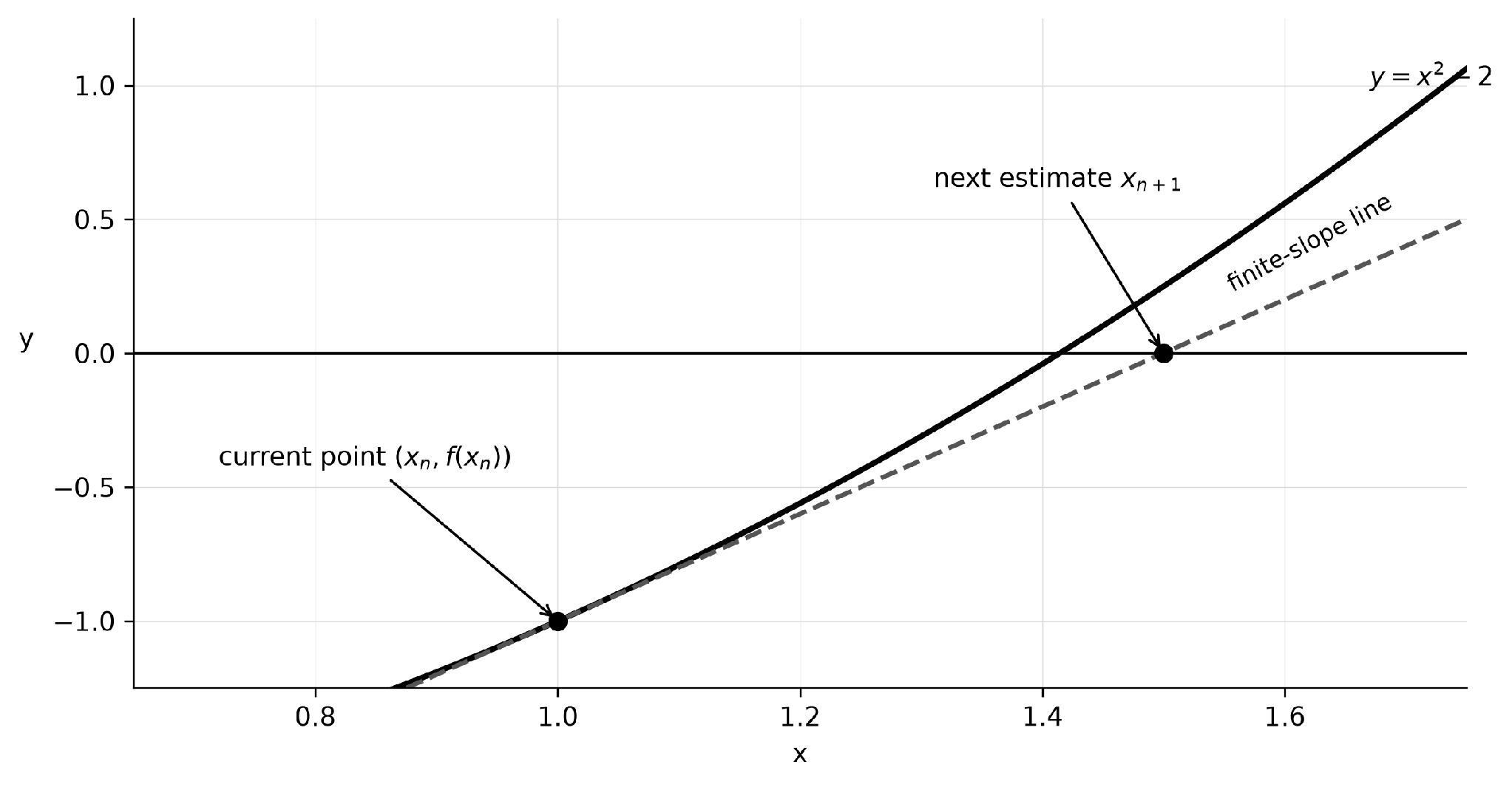
Table 2. Newton-style finite-slope correction with h = 0.001.
| Iteration | Current estimate, xₙ | f(xₙ) | Finite slope, mₙ | Next estimate, xₙ₊₁ | Correction | Residual | Absolute error |
|---|---|---|---|---|---|---|---|
| 0 | 1.000000 | −1.000000 | 2.001000 | 1.499750 | 0.499750 | 0.249250 | 0.085537 |
| 1 | 1.499750 | 0.249250 | 3.000500 | 1.416680 | 0.083070 | 0.006984 | 0.002467 |
| 2 | 1.416680 | 0.006984 | 2.834361 | 1.414217 | 0.002464 | 8.53 × 10⁻⁶ | 3.02 × 10⁻⁶ |
| 3 | 1.414217 | 0.000009 | 2.829433 | 1.414214 | 0.000003 | 3.03 × 10⁻⁹ | 1.07 × 10⁻⁹ |
The correction is |xₙ₊₁ − xₙ|, the residual is |f(xₙ₊₁)|, and the absolute error is measured relative to √2. All decrease sharply across the verified iterations.
Newton's Method offers an example of repeated correction. Classroom discussion should then return to Leibniz because the Calculus Abacus originated from a project centered on Nova Methodus, and relations among differences remain the principal historical connection. Newton supports one stage of the teaching sequence rather than replacing the Leibniz-centered framework.
What the Abacus Can and Cannot Show
The abacus is strongest when construction carries meaning. Setup teaches representation: students learn how floor, increment, stone value, and the size-curve encode a function. Play teaches mathematical action: they compare neighboring columns, build the change-curve, estimate slopes and areas, refine increments, and correct provisional roots. Manual work builds familiarity with concepts. Formalization becomes useful after students understand the actions that a rule, formula, or notation will express.
The abacus displays finite calculations. It can show why a narrower interval may improve a local estimate, why an area contribution needs a width, and why a root correction may overshoot before settling. It cannot prove convergence, turn finite differences into infinitesimals, reproduce Wallis's quadrature, enact Fermat's adequality, or establish Leibniz's foundations. Those limits keep each historical comparison precise.
The three companion exercises follow naturally from these distinctions. Students first build an area from finite contributions and compare brackets. Next they turn neighboring changes into rates and compare two-sided estimates. Finally, they use a local rate to correct an estimated root. Teachers can ask what makes each new estimate more trustworthy. The answer changes with the task: the area bracket narrows, the slope estimates close from two sides, or the root residuals shrink. These parallels do not imply that the historical mathematicians shared a single method.
Teacher Reflection
- What evidence would persuade students that an estimate has become more reliable?
- How does repeated refinement help students distinguish an emerging target value from any one estimate calculated with a finite increment?
- When does the historical analogy help students understand the mathematics, and when does it stop being useful?
Conclusion
The four historical connections highlight different aspects of early calculus. Wallis connects arithmetic patterns and finite columns with the problem of determining area. Fermat focuses attention on nearby expressions and residual terms. Leibniz places differences and their relations at the center of a calculus for tangents, maxima, and minima. Newton's numerical work supports iterative correction of a provisional root.
In the classroom, these connections form a practical sequence: calculate finite differences and notice patterns of change; divide by the increment and refine a tangent estimate; multiply column heights by widths and compare area estimates; use a local slope to correct a root; then decide whether the results are settling. The Calculus Abacus does not recreate the origins of calculus. It lets students carry out several mathematical actions that compact notation can otherwise hide.
Notes
¹ Jeffrey Elawani, Leibniz's Science of Estimation: A Measure for the Synthesis of Universal Mathematics, Dynamics, and Metaphysics, unpublished doctoral thesis draft used with permission (2026), Abstract. The source is cited only for this historical meaning of estimation.
² John Wallis, Arithmetica Infinitorum (Oxford, 1656), https://doi.org/10.3931/e-rara-38681.
³ Gottfried Wilhelm Leibniz, "A New Method for Maxima and Minima," translated by Dirk J. Struik, in A Source Book in Mathematics, 1200–1800 (1986), pp. 271–281.
⁴ Arthur and Rabouin distinguish finite and infinitely small readings of the historical terminology. Section 5.2 (pp. 111–118) examines quantity and magnitude; Section 6.3 (pp. 149–152) examines justification of the algorithm. Their translated extract of the 1684 paper appears on pp. 201–204. See https://doi.org/10.1007/978-3-031-77259-7.
⁵ The Newton Project record NATP00204 dates the manuscript 31 July 1669 and identifies its numerical resolution of affected equations. Ypma traces the later method in SIAM Review, 37(4), pp. 531–551, https://doi.org/10.1137/1037125.
References
Arthur, R. T. W., & Rabouin, D. (2025). Leibniz on the foundations of the differential calculus. Birkhäuser.
Breger, H. (1994). The mysteries of adaequare: A vindication of Fermat. Archive for History of Exact Sciences, 46(3), 193–219.
Elawani, J. (2026). Leibniz's science of estimation: A measure for the synthesis of universal mathematics, dynamics, and metaphysics [Unpublished doctoral thesis draft].
Fermat, P. de. (1679). Varia Opera Mathematica. Jean Pech.
Giusti, E. (2009). Les méthodes des maxima et minima de Fermat. Annales de la Faculté des sciences de Toulouse, 18(S1), 59–85.
Katz, M. G., Schaps, D. M., & Shnider, S. (2013). Almost equal: The method of adequality from Diophantus to Fermat and beyond. Perspectives on Science, 21(3), 283–324.
Leibniz, G. W. (1986). A new method for maxima and minima, as well as tangents (D. J. Struik, Trans.). In D. J. Struik (Ed.), A source book in mathematics, 1200–1800 (pp. 271–281). Princeton University Press. (Original work published 1684).
Newton, I. (1669). De Analysis per aequationes numero terminorum infinitas [Manuscript]. The Newton Project.
Wallis, J. (1656). Arithmetica Infinitorum. Leonard Lichfield.
Ypma, T. J. (1995). Historical development of the Newton-Raphson method. SIAM Review, 37(4), 531–551.
Written for the Calculus Abacus Project by Hamza Amin, with AI assistance, 2026.