Correct the Guess
Students use current error and a local slope estimate to construct tangent-style corrections toward √2, then judge whether the provisional roots are stabilizing.
Exercise 3 · Estimation Before Formalization Companion Exercises
Learning Objective
Students will interpret root finding as iterative correction, construct the next estimate from the x-intercept of a local line, compare exact-function and stone-reconstructed values, and identify quantitative evidence of stabilization.
Teacher Overview
This exercise follows the article’s discussion of Newton’s Method. It begins with a geometric question: if a locally straight line continues to the x-axis, where does it land? Students use the abacus to obtain a finite forward slope and a function value, calculate the intercept, and repeat.
The exercise draws on Newton’s idea of correcting an estimate, although the classroom procedure is modern. Newton’s work included numerical correction of equations, but he did not use this interface or this exact sequence.
Student Activity
Setup and app sequence
Choose Show panels. Set formula x^2 - 2, midpoint 1, increment 0.01, and max stones 50. Enable Fractional stones and 10 decimals; then select Fill Board and Find Differences, which generates the change-size stones. For every new midpoint, refill and select Find Differences again. Record the app’s floor and stone value each time because the display rescales when the window changes.
PREDICT. The root of x² − 2 lies between 1 and 2. Starting at x₀ = 1, the function value is negative and the local slope is positive. Should the correction move left or right? Should it travel all the way to 2? Explain from a sketch.
CONSTRUCT A LOCAL LINE. Use Figure 1 as the geometric model. With h = 0.01, record f(1) and f(1.01). Calculate
m₀ = [f(1.01) − f(1)]/0.01.
The local line through (x₀, f(x₀)) has equation
y − f(x₀) = m₀(x − x₀).
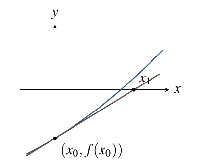
Figure 1: The finite-slope line through the current point meets the axis at the next estimate.
Set y = 0, solve for the line’s x-intercept, and call it x₁. Do not use the standard Newton formula yet; reason from the line.
CHECK THE DIRECTION. Evaluate f(x₁). Is the new point left or right of the true root? How does the sign of f(x₁) tell you?
REPEAT. Enter the displayed rounded midpoint 1.4975, keeping h = 0.01. Record the forward slope estimate. Calculate f(1.4975) from the formula, construct the new local line, and find x₂. Repeat once more using x₂ rounded to 1.4168.
| step | xₙ | f(xₙ) | slope mₙ | xₙ₊₁ | correction | residual | abs. error |
|---|---|---|---|---|---|---|---|
| 0 | 1.0000 | ||||||
| 1 | 1.4975 | ||||||
| 2 | 1.4168 |
Here correction means |xₙ₊₁ − xₙ|, residual means |f(xₙ₊₁)|, and absolute error means |xₙ₊₁ − √2|.
COMPARE REPRESENTATIONS. The app may show a rounded fractional stone count. Reconstruct f(xₙ) from the signed stone count and the displayed stone value, accounting for the floor if required. Compare that reconstruction with direct substitution into x² − 2. Which should you use for a reproducible mathematical check? Which better represents what a student literally reads from the board?
JUDGE STABILIZATION. Compare successive estimates with √2 ≈ 1.4142135624. Record the absolute error and the size of each correction. State a practical stopping rule before looking at the last row, then decide when to stop.
Reflection Questions
- How do the sign of the function value and the sign of the slope determine the correction’s direction?
- Which is better evidence of stabilization: many matching displayed digits, a small residual f(xₙ), or a small correction? What does each show?
- Why can a rounded stone reconstruction and direct function evaluation give slightly different next estimates without invalidating the method?
Teacher Discussion Extension
Only after students have built at least two intercepts, derive the compact recurrence. Setting y = 0 in the local-line equation gives
xₙ₊₁ = xₙ − f(xₙ)/mₙ.
If the local slope is represented by the derivative, this becomes the standard textbook formula. Here mₙ remains a forward finite slope with h = 0.01, which explains a small systematic difference from an exact-tangent iteration.
As an optional extension, use f(x) = sin x, x₀ = 3, and h = 0.001. The first finite-slope update is approximately 3.1425364078; the second is approximately 3.1415926527, close to π. Confirm radian mode through the app’s validated behavior.
What Students Often Notice
- The first correction overshoots, but the next correction is much smaller.
- The function value can be small even when the displayed stack is not, because scale and floor govern representation.
- A stable-looking midpoint is more persuasive when the residual and correction size also shrink.
- The slope need not be perfect for the correction to improve the estimate.
Expected Student Discoveries
Root estimation works here as a feedback process. Students measure the current error, use local steepness to convert vertical error into a horizontal correction, and then test the new value. Converging estimates, smaller corrections, and smaller residuals provide stronger grounds for stopping than the curve’s appearance alone.
Common Misconceptions
- Using the slope as the correction. The vertical error must be divided by slope to obtain a horizontal correction.
- Ignoring sign. The subtraction in the intercept construction carries direction; replacing every quantity by a magnitude can move away from the root.
- Forgetting the floor. A stack is relative to the displayed baseline. Direct substitution is the clean check.
- Treating rounded agreement as proof. A stopping rule is a practical judgment, not a convergence proof.
Teacher Notes and Mathematical Check
At x₀ = 1, f(x₀) = −1, m₀ = 2.01, and
x₁ = 1 − (−1)/2.01 = 1.497512437810945… .
Using the rounded midpoint 1.4975,
f(1.4975) = 0.24250625, m₁ = 3.005, x₂ = 1.416799084858569… .
Using the rounded midpoint 1.4168,
f(1.4168) = 0.00732224, m₂ = 2.8436, x₃ = 1.414225010550007… .
The errors relative to √2 are approximately 0.08330, 0.002586, and 0.00001145. The complete check is:
| step | xₙ | f(xₙ) | mₙ | xₙ₊₁ | correction | residual | abs. error |
|---|---|---|---|---|---|---|---|
| 0 | 1.0000 | −1 | 2.01 | 1.49751244 | 0.49751244 | 0.24254350 | 0.08329888 |
| 1 | 1.4975 | 0.24250625 | 3.005 | 1.41679908 | 0.08070092 | 0.00731965 | 0.00258552 |
| 2 | 1.4168 | 0.00732224 | 2.8436 | 1.41422501 | 0.00257499 | 0.00003238 | 0.00001145 |
If a reconstructed display gives f(1.4975) ≈ 0.2427, the next value is 1.4167346090, a difference caused by display rounding rather than a change in the intercept idea.
Connection to the Historical Article
The article presents Newton-style root finding as repeated correction of an estimated value. Students construct the tangent-intercept idea before they meet the compact formula. The finite visualization is associated with Newton’s Method, but it does not reconstruct Newton’s manuscript procedure.
Classroom Timing and Adaptation
Allow five minutes for the geometric prediction, fifteen for the first two intercepts, ten for the representation comparison, and ten for stabilization and discussion. Have pairs alternate between “app reader” and “line calculator” so that no student treats the displayed slope as an unexplained answer.
For additional support, provide a diagram of a rising line through a point below the axis and ask students to mark the intercept before using numbers. For additional challenge, compare the finite-slope correction with an exact-tangent correction at the same midpoint and explain the discrepancy. The optional sine extension is best reserved for a group that can work confidently in radians.
Quick Formative Assessment
Give students f(xₙ) = −0.08 and a positive local slope estimate mₙ = 2.5. Without completing an iteration, ask for the correction’s direction and approximate size. A successful answer says the estimate should move right by about 0.08/2.5 = 0.032 and explains the sign rather than relying on a memorized formula.
Written for the Calculus Abacus Project by Hamza Amin, with AI assistance, 2026.